R Function of the Day: foodweb

The R Function of the Day series will focus on describing in plain language how certain R functions work, focusing on simple examples
that you can apply to gain insight into your own data.

Today, I will discuss the foodweb function, found in the mvbutils
package.

Foodweb? What is that?

In biology, a foodweb is a group of food chains, showing the complex
relationships that exist in nature. Similarly, the R foodweb
function contained in the mvbutils package on CRAN displays a
flowchart of function calls. What functions does my function call?
What funtions in my package call the lm function? These are the
types of questions that can be answered in a graphical way using
foodweb. This information can be useful for documenting your own
code, and for learning how a package that you’re not familiar with
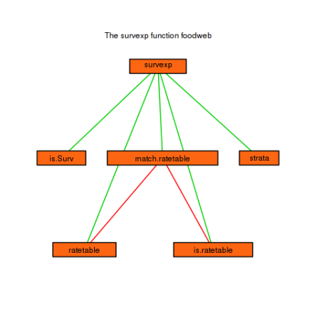
works. At the end of this post, you’ll see an example with a diagram
of the survexp function from the survival package.

First, you have to install and load the mvbutils package, so let’s
do that first.

install.packages("mvbutils")
library(mvbutils)

A simple example

Let’s define a couple simple functions to see how foodweb works. We
simply define a function called outer that calls two functions,
inner1 and inner2.

inner1 <- function() {
  "This is the inner1 function"
}

inner2 <- function() {
  "This is the inner2 function"
}

outer <- function(x) {
   i1 <- inner1()
   i2 <- inner2()
}  

Now let’s use the foodweb function to diagram the relationship between
the outer and inner functions. If we don’t give foodweb any
arguments, it will scour our global workspace for functions, and make
the diagram. Since the only functions in my global workspace are the
ones we’ve just defined, we get the following plot.

foodweb()

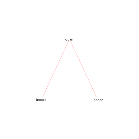
We see a simple graph showing that the outer function calls both the
inner1 and inner2 functions, jus as we expect. We can make this look a
bit nicer by adjusting a few of the arguments.

foodweb(border = TRUE, expand.xbox = 3,
        boxcolor = "#FC6512", textcolor = "black",
        cex = 1.2, lwd=2)

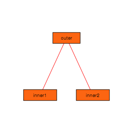
You can see that you can control many of the graphical parameters of
the resulting plot. See the help page for foodweb to see the
complete list of graphical parameters you can specify.

A more complicated example

As we saw above, by default foodweb will look in your global
workspace for functions to construct the web from. However, you can
pass foodweb a group of functions to operate on. There are several
ways of doing this, see the help page for examples. The code below
shows one possiblity, when we want to limit our results to functions
appearing in a specific package. The prune argument is very useful.
It takes a string (or regular expression) to prune the resulting graph
to.

foodweb(where = "package:survival", prune = "survexp",
        border = TRUE,
        expand.xbox = 2, boxcolor = "#FC6512",
        textcolor = "black", cex = 1.0, lwd=2)
mtext("The survexp function foodweb")

Conclusion

I have used the foodweb function to help understand other user’s
code that I have inherited. It has proved very valuable in aiding the
comprehension of hard to read or complicated functions. I have also
used it in the development of my own packages, as it sometimes can
suggest ways to reorganize the code to be more logical.

Introduction to using R with org-babel, Part 1

In my opinion, the description of orgmode by its creator as a tool “for keeping notes, maintaining ToDo lists, doing project planning, and authoring with a fast and effective plain-text system” is a little like describing Emacs as a “text editor”. While technically accurate, one not acquainted with orgmode might not be immediately persuaded to learn it based on its pedestrian description. Needless to say, I think it is worthwhile.

While there are plenty of tutorials and a great introduction to orgmode on its site, there exists a relatively new orgmode extension called org-babel whose documentation, although complete and accurate, might benefit from a high-level overview showing how it can be used to write an R program in an orgmode buffer.

What can orgmode do with source code?

Even without org-babel, you can create a source code block in an orgmode buffer. Why would you want to do this? Mostly so that when you export the orgmode buffer to HTML, that the source code looks like source code. Source code will be displayed in a monospace font, and colored to look just like it does in your Emacs buffer.

To accomplish this, you would put something like the following in your org-mode document. I will use the programming language R as an example. To define a source code block, simply use the #+BEGIN_SRC syntax along with the major mode of the language, in this case ‘R’.

#+BEGIN_SRC R
x <- 1:5

square <- function(x) {
  x^2
}

square(x)
#+END_SRC

Then, when you export the orgmode document to, say, HTML, your R code will look just as it does in Emacs with syntax highlighting, and will be offset from the text surrounding it, like this:

x <- 1:5

square <- function(x) {
  x^2
}

square(x)

A note about syntax highlighting in Emacs

Ideally, when you entered into a code block, Emacs would recognize this, and the syntax highlighting within the code block would reflect whatever language you had specified as you typed it. Unfortunately, it is difficult to get Emacs to behave this way, at least with orgmode. I have investigated several options for doing this, but have run into problems with all of them. Orgmode’s solution to this is to create an indirect buffer containing the source code you’re editing when you type C-c ‘ (i.e., Control-C, then a single quote) in a source code block. You don’t have to do this, but it is nice to get your program in a temporary buffer that is set to the right mode. In R, this also means you can use all the usual ESS shortcut keys.

What does org-babel add to what orgmode can already do?

Org-babel lets you execute source code blocks in an orgmode buffer. Well, what does that mean? At its simplest, org-babel lets you submit a source code block, like the one above, to an R process, and places the results in the actual orgmode buffer.

You activate the additional features that org-babel provides by giving the #+BEGIN_SRC line in an orgmode buffer special arguments, some of which I describe below. All the available options are described in the org-babel documentation. I will show some basic examples of how to add arguments to a #+BEGIN_SRC line.

However, since submitting a code block to a new R process and placing the results in the orgmode buffer is the default behavior of org-babel, you don’t need to supply any arguments to the source code block for this simple operation. You simply carry out this process by typing C-c C-c in a source code block.

#+BEGIN_SRC R
x <- 1:5

square <- function(x) {
  x^2
}

square(x)
#+END_SRC

In your org-mode buffer, with point in the code block, you now type C-c C-c, an R process is started, and the following is placed in the orgmode buffer.

#+results: |  1 | |  4 | |  9 | | 16 | | 25 |

Since we used the default value for the results argument (i.e., we didn’t specify anything), org-babel collected the output and put it in an org-table, as shown above. If you just want the output like it would appear in your ESS R process buffer, you can use the value ‘output’ to the results argument, as shown below. You specify an argument by typing a ‘:’, and then using one of the valid parameter names, typing a space, and then giving the value of the parameter. So, in the example below, results is the name of the parameter, and we’re setting its value to ‘output’. The default value for the results parameter is ‘value’, and gives you the same results as above, i.e., a table of the last results returned by the code block.

#+BEGIN_SRC R :results output
x <- 1:5

square <- function(x) {
  x^2
}

square(x)
#+END_SRC

#+results: : [1]  1  4  9 16 25 

Since we set results to ‘output’, we see the familiar R notation for printing a vector. The default value, where an org-table is created, would be useful for passing the resulting table to perhaps a different function within the orgmode buffer, even one programmed in another language. That is a feature that org-babel supports and encourages, but I will not describe that further here.

Personally, I set results to ‘output’ to write this entries for this blog, since it shows users what the actual R output will look like. This is nice, because there is no cutting and pasting of the results! I can just write my R code in a source code block, and then add a special argument to export the code and results to an HTML file upon exporting in orgmode. My code block would look like this to accomplish that. Notice the new argument, exports, and its value ‘both’, as in both the code and its results.

#+BEGIN_SRC R :results output :exports both 
x <- 1:5

square <- function(x) {
  x^2
}

square(x)
#+END_SRC

Putting the above code in an orgmode buffer and exporting to HTML will show the following:

x <- 1:5

square <- function(x) {
  x^2
}

square(x)

[1]  1  4  9 16 25

Indeed, using org-babel in this fashion is how I now generate content for this site. Compare this approach to what I used to be doing with Sweave. The two approaches are similar, but I now have a completely contained orgmode approach, where as before I had to preprocess the orgmode buffer with an Sweave function before export. You can see the difference not only in how I specify code blocks, but also how the appearance of the output has changed.

Note that the last thing I still have to do in an Elisp function is to insert inline CSS code to generate the background color and outline of the code and results blocks. As far as I know, there is no way to do this in orgmode yet, as the HTML output it contains the CSS style information in the HTML header.

Why do things this way?

I think org-babel is interesting for several reasons. First, as R was one of the first languages supported by it, and I use R as my main programming language at my job, I was naturally interested in it. Org-babel is very useful for me because I am used to working in orgmode, so I can add links, tags, TODO items, create notes, and more right in my code. It’s like having a hyper-commenting system that can be crosslinked with everything. Using orgmode’s intuitive visibility cycling system results in a powerful code-folding feature. Orgmode properties allow me to collect meta-information about my code, such as what objects a code block create.

The export feature of orgmode is very useful for producing this blog, and producing readable documentation for my source code. Also, if I am writing a program to be run in a script, a very common task, org-babel can handle that through a feature called tangling, which I will cover in a future article. The tangling feature turns orgmode into a tool to perform literate programming.

What is left to cover?

In addition to tangling mentioned above, there are several important features that I have not even mentioned in this short introduction. In the subsequent article, I want to show how I use R with org-babel to include inline images created with R, and how to generate output that can be previewed inline in orgmode documents. Using org-babel in this manner closely mirrors a ‘notebook’ style interactive session such as Mathematica provides. The other main feature that org-babel provides is using it as a meta-programming language to, say, call R functions using data generated from a shell script or Python program. Org-babel is a very interesting project that is definitely worth your time to check out, especially if you’re already an Emacs or orgmode user. If you’ve read through this post, you can get started by reading the official org-babel introduction, which will describe what to include in your .emacs file to setup org-babel.

R Function of the Day: sample

The R Function of the Day series will focus on describing in plain language how certain R functions work, focusing on simple examples
that you can apply to gain insight into your own data.

Today, I will discuss the sample function.

Random Permutations

In its simplest form, the sample function can be used to return a
random permutation of a vector. To illustrate this, let’s create a
vector of the integers from 1 to 10 and assign it to a variable x.

x <- 1:10

Now, use sample to create a random permutation of the vector x.

sample(x) 

 [1]  3  2  1 10  7  9  4  8  6  5

Note that if you give sample a vector of length 1 (e.g., just the
number 10) that it will do the exact same thing as above, that is,
create a random permutation of the integers from 1 to 10.

sample(10) 

 [1] 10  7  4  8  2  6  1  9  5  3

Warning!

This can be a source of confusion if you’re not careful. Consider the
following example from the sample help file.

sample(x[x > 8])
sample(x[x > 9])

[1] 10  9
 [1]  9  3  4  8  1 10  7  5  2  6

Notice how the first output is of length 2, since only two numbers are
greater than eight in our vector. But, because of the fact that only
one number (that is, 10) is greater than nine in our vector, sample
thinks we want a sample of the numbers from 1 to 10, and therefore
returns a vector of length 10.

The replace argument

Often, it is useful to not simply take a random permutation of a
vector, but rather sample independent draws of the same vector. For
instance, we can simulate a Bernoulli trial, the result of the flip of
a fair coin. First, using our previous vector, note that we can tell
sample the size of the sample we want, using the size argument.

sample(x, size = 5)

[1]  2 10  5  1  6

Now, let’s perform our coin-flipping experiment just once.

coin <- c("Heads", "Tails")
sample(coin, size = 1)

[1] "Tails"

And now, let’s try it 100 times.

sample(coin, size = 100)

Error in sample(coin, size = 100) : 
  cannot take a sample larger than the population when 'replace = FALSE'

Oops, we can’t take a sample of size 100 from a vector of size 2,
unless we set the replace argument to TRUE.

table(sample(coin, size = 100, replace = TRUE))

Heads Tails 
   53    47

Simple bootstrap example

The sample function can be used to perform a simple bootstrap.
Let’s use it to estimate the 95% confidence interval for the mean of a
population. First, generate a random sample from a normal
distribution.

rn <- rnorm(1000, 10)

Then, use sample multiple times using the replicate function to
get our bootstrap resamples. The defining feature of this technique is
that replace = TRUE. We then take the mean of each new sample, gather them, and finally compute the relevant quantiles.

quantile(replicate(1000, mean(sample(rn, replace = TRUE))),
         probs = c(0.025, 0.975))

     2.5%     97.5% 
 9.936387 10.062525

Compare this to the standard parametric technique.

t.test(rn)$conf.int

[1]  9.938805 10.061325
attr(,"conf.level")
[1] 0.95

Making Emacs Buffer Names Unique Using the Uniquify Package

If you ever work in Emacs with different files that all have the same name, this tip may be very useful for you. In my experience, this most often happens when working with Makefiles from multiple projects or directories. Assuming you have a buffer visiting a file called Makefile, by default Emacs will call the second buffer Makefile<2>. This is not very useful for figuring out which one is which.

The uniquify package

Enter the uniquify package. It offers several options for making buffer names unique. In my .emacs, I have the following two lines of code.

(require 'uniquify)
(setq uniquify-buffer-name-style 'forward)

You can set the value to any of the following options, nil being the default. These examples are taken from the help file within Emacs. They use the information from the directories the files are located in to make the names unique. The first buffer called “name” is visiting a file in the directory bar/mumble/, and the second buffer is visiting a file called “name” in directory quux/mumble.

value	first buffer called “name”	second buffer called “name”
forward	bar/mumble/name	quux/mumble/name
reverse	name\mumble\bar	name\mumble\quux
post-forward	name|bar/mumble	name|quux/mumble
post-forward-angle-brackets	name<bar/mumble>	name<quux/mumble>
nil	name	name<2>

Using R to Analyze Baseball Games in “Real Time”

In order to honor the last day of the 2009 MLB regular season (excepting the Twins/Tigers tiebreaker Tuesday night), I was reading a book that combines a few of my favorite thing: statistics, R, and baseball. The book, by Joseph Adler, is called Baseball Hacks, and I highly recommend it if you are interested in analyzing baseball data. Joseph uses Excel for some tips, R for others, and shows you how to download historical and current baseball data for further analysis. One tip that the book offered was a way to download “real time” baseball data from MLB’s site in XML format. I decided to try to write some R functions to retrieve, summarize, and analyze what was available.

Where are the data?

Joseph shows how, at least at the time of the writing of his book and this post, you can go here to download a wealth of XML data from past and current seasons. If you drill down far enough into the directories, you can find a file called miniscoreboard.xml, which is the one I use for this analysis.

The R functions

Here are the R functions I wrote. You can copy and paste them into your R session so that they are available to you. The next section will describe how to use them. Writing these was fairly straightforward, and simply a matter of XML manipulation. I admit that there may be far better ways to do this manipulation using the XML package, but this worked for now.

################################################################################
#   Program Name:     xml-mlb-gameday.R
#   Author:           Erik
#   Created:          10/04/2009
#
#   Last saved
#    Time-stamp:      <2009-10-04 17:23:02 erik>
#
#   Purpose:          show current scoreboard in R 
#
#   ** Generated by auto-insert on 10/04/2009 at 13:25:58**
################################################################################

## need XML package, may need to install w/ install.packages()
library(XML)

## create a boxscore object from an XML description of a game 
createBoxScore <- function(x) {
  status <- if(x$.attrs["status"] != "In Progress")
    "Final" else if(x$.attrs["top_inning"] == "Y")
      "Top" else "Bot"
  
  bs <- list(status = status, 
             inning = as.numeric(x$.attrs["inning"]),
             away.team = x$.attrs["away_name_abbrev"],
             away.runs = as.numeric(x$.attrs["away_team_runs"]),
             away.hits = as.numeric(x$.attrs["away_team_hits"]), 
             away.errors = as.numeric(x$.attrs["away_team_errors"]),
             home.team = x$.attrs["home_name_abbrev"],
             home.runs = as.numeric(x$.attrs["home_team_runs"]), 
             home.hits = as.numeric(x$.attrs["home_team_hits"]), 
             home.errors = as.numeric(x$.attrs["home_team_errors"]))
  class(bs) <- "boxscore"
  bs
}

## print the boxscore object in traditional format
print.boxscore <- function(x, ...) {
  cat("     ", "R   ", "H  ", "E (",
      x$status, " ",
      x$inning, ")\n",
      format(x$away.team, width = 3), " ", 
      format(x$away.runs, width = 2), "  ", 
      format(x$away.hits, width = 2), "  ", 
      x$away.errors, "\n",
      format(x$home.team, width = 3), " ", 
      format(x$home.runs, width = 2), "  ", 
      format(x$home.hits, width = 2), "  ", 
      x$home.errors, "\n\n", sep = "")
}

## utility function ... 
as.data.frame.boxscore <- function(x, row.names, optional, ...) {
  class(x) <- "list"
  as.data.frame(x)
}

## This is the "user accessible" public function you should be calling!
## downloads the XML data, and prints out boxscores for games on "date"
boxscore <- function(date = Sys.Date()) {
  if(date > Sys.Date())
    stop("Cannot retrieve scores from the future.")
         
  year  <- paste("year_", format(date, "%Y"), "/", sep = "")
  month <- paste("month_", format(date, "%m"), "/", sep = "")
  day   <- paste("day_", format(date, "%d"), "/", sep = "")
         
  xmlFile <-
    paste("http://gd2.mlb.com/components/game/mlb/",
          year, month, day, "miniscoreboard.xml", sep = "")
  xmlTree <- xmlTreeParse(xmlFile, useInternalNodes = TRUE)
  xp <- xpathApply(xmlTree, "//game")
  xmlList <- lapply(xp, xmlToList)

  bs.list <- lapply(xmlList, createBoxScore)
  names(bs.list) <-
    paste(sapply(bs.list, "[[", "away.team"),
                 "@",
          sapply(bs.list, "[[", "home.team"))
  bs.list
}

Examples of summarizing real-time baseball data

Here is how to run some simple analyses on baseball games happening right now. This is the real value add for the idea of downloading data through R. Obviously you could just go to your favorite sports site to find scores if you wanted to know how your team was doing, but pulling the data into R lets you further analyze the data, and even combine it with other data sources (e.g., weather).

> ## print boxscores for games happening NOW!
> boxscore()
$`CWS @ DET`
     R   H  E (Final 9)
CWS  3   7  0
DET  5  12  0


$`HOU @ NYM`
     R   H  E (Final 9)
HOU  0   4  1
NYM  4   9  0


$`PIT @ CIN`
     R   H  E (Final 9)
PIT  0  10  0
CIN  6  11  0


$`WSH @ ATL`
     R   H  E (Final 15)
WSH  2  13  0
ATL  1  13  0


$`CLE @ BOS`
     R   H  E (Final 9)
CLE  7   8  0
BOS 12  11  0


$`FLA @ PHI`
     R   H  E (Final 10)
FLA  6  11  1
PHI  7  12  0


$`TOR @ BAL`
     R   H  E (Final 11)
TOR  4   9  2
BAL  5   8  0


$`NYY @ TB`
     R   H  E (Final 9)
NYY 10  12  0
TB   2   7  2


$`KC @ MIN`
     R   H  E (Final 9)
KC   4  12  0
MIN 13  11  0


$`MIL @ STL`
     R   H  E (Final 10)
MIL  9  15  2
STL  7   7  0


$`ARI @ CHC`
     R   H  E (Final 9)
ARI  5   8  0
CHC  2   6  0


$`LAA @ OAK`
     R   H  E (Final 9)
LAA  5   9  1
OAK  3  12  1


$`SF @ SD`
     R   H  E (Bot 9)
SF   3  11  1
SD   3   4  0


$`COL @ LAD`
     R   H  E (Top 8 )
COL  1   4  1
LAD  5  12  0


$`TEX @ SEA`
     R   H  E (Final 9)
TEX  3   4  0
SEA  4   8  1 
> ## print boxscores for a different day's games
> boxscore(date = as.Date("2009-10-01"))
$`STL @ CIN`
     R   H  E (Final 9)
STL 13  15  1
CIN  0   5  0


$`MIN @ DET`
     R   H  E (Final 9)
MIN  8  13  4
DET  3   7  1


$`MIL @ COL`
     R   H  E (Final 9)
MIL  2   6  0
COL  9  14  1


$`ARI @ SF`
     R   H  E (Final 9)
ARI  3   6  1
SF   7  11  0


$`TEX @ LAA`
     R   H  E (Final 9)
TEX 11  15  1
LAA  3   7  2


$`WSH @ ATL`
     R   H  E (Final 9)
WSH  2   7  0
ATL  1   6  0


$`HOU @ PHI`
     R   H  E (Final 9)
HOU  5  10  0
PHI  3  13  1


$`BAL @ TB`
     R   H  E (Final 9)
BAL  3   7  0
TB   2   5  1


$`CLE @ BOS`
     R   H  E (Final 9)
CLE  0   3  0
BOS  3  12  0


$`PIT @ CHC`
     R   H  E (Final NA)
PIT NA  NA  NA
CHC NA  NA  NA


$`OAK @ SEA`
     R   H  E (Final 9)
OAK  2   7  1
SEA  4   8  0 
> ## save the boxscores for futher analysis
> bs <- boxscore()
> ## convert to a more useful form, a data.frame
> ## with one game per row 
> bs.df <- do.call(rbind, lapply(bs, as.data.frame))
> ## status of today's games
> table(bs.df$status)
Final   Bot   Top 
   13     1     1  
> ## how many innings have been played today? 
> sum(bs.df$inning, na.rm = TRUE)
[1] 144 
> ## how many runs have been scored by the home teams today?
> sum(bs.df$home.runs, na.rm = TRUE)
[1] 79 
> ## how many runs have been scored by the away teams today?
> sum(bs.df$away.runs, na.rm = TRUE)
[1] 62 

Conclusion

These functions are far from robust, and I think they only work for the current year (i.e., 2009, dates from 2008 were not working right). The format looks like it has changed over time, which is not surprising. I only use a very small subset of the available data, even the miniscoreboard.xml file contains far more information than I summarize here. This is really the first time I have dealt with XML data, so I am sure there is a lot more that can be done, but for a one-day project, I think the results are pretty interesting. I will definitely provide the updates I make to these functions, and may even start a baseball R package if they grow extensive enough. I suppose this is a project I can work on in the off season!

Using doc-view with auto-revert to view LaTeX PDF output in Emacs

When I am authoring a document in Emacs, such as a report or my CV, it is useful for me to compile the source file periodically to see what the resulting file PDF looks like. I used to run a separate PDF viewer to look at the output, but I now have a complete Emacs solution.

The editing environment

When writing a document, I usually want the output to be a PDF file. Accordingly, I put the following in my .emacs file.

(setq TeX-PDF-mode t)

I then split my Emacs frame into two buffers vertically, using C-x 3 (see screencast below). After compiling my file with C-c C-c, I visit the resulting PDF file in the other Emacs window. The Emacs doc-view package will display the PDF file.

Including auto-revert functionality

The final piece to the puzzle is to set files visited in doc-view-mode to auto-revert when changed on disk. That way, then I update my file and recompile with C-c C-c, the PDF in the other window will automatically update.

This is achieved by placing the following line in my .emacs.

(add-hook 'doc-view-mode-hook 'auto-revert-mode)

Screencast Example

Here is a screencast of this process in action.

This is a simple setup that I use to author reports, edit them, and see immediate updates to my output file without leaving Emacs.

R Object Tooltips in ESS

Whether at work or for personal projects, I use ESS a lot to perform interactive data analyses. The ability to write, edit, and submit R commands to an interactive R process is simply something I cannot imagine analyzing data without.

An example

One thing that I end up having to do a lot is inspect an object that I have just assigned to a variable in R. To fix ideas, let us create a data.frame called df for this example.

> df <- data.frame(patient = 1:100,
                   age = rnorm(100, mean = 10, sd = 6),
                   sex = sample(gl(2, 50, labels =
                     c("Male", "Female"))))

I just created the data.frame df, and I want to know if I did it correctly. For instance, does it look like I expect it to? Does it have 100 observations like I want? Do the variables have the right names? Is the sex variable a factor with two levels? In short, I want to call the str function using the object df as an argument.

Here is the output I am interested in seeing:

> str(df)
'data.frame':   100 obs. of  3 variables:
 $ patient: int  1 2 3 4 5 6 7 8 9 10 ...
 $ age    : num  11.06 7.73 17.61 3.11 6.76 ...
 $ sex    : Factor w/ 2 levels "Male","Female": 2 1 1 2 2 1 1 2 2 2 ... 

Inspecting objects the old way

So, how can I quickly see the structure as shown above? One idea is to switch over to my interactive R buffer in Emacs, type the command at the prompt, and then switch back to my code buffer to edit the data.frame command or continue programming. I dislike having to switch back and forth between the buffers for a one-off command though.

Alternatively, I could type str(df) in my code buffer, evaluate it, and decide to keep it or delete the line. Since this is more of a quick check, without permanent results, I usually will not want to keep lines like this around, since they clutter up my program. Typically, I am writing the program to be later run in BATCH mode, so I also do not want functions like that in my code since some can be excessively time-consuming depending on the size of the data.frame.

Another option is to use the ESS function ess-execute-in-tb, by default this is bound to C-c C-t, which will prompt me for an expression to evaluate. This is nice because I do not have to clutter my buffer with extraneous function calls. However, after using this method for a while, I noticed that I had many patterns with my objects. For data.frames, I would almost always use summary or str on them after assignment. For factors, I would want to table the values after I created them, to be sure they looked right. For numeric vectors, I would want to summarize them. I also wanted to summarize model fits (e.g., lm). I wanted to take advantage of my usage patterns so that I did not have to type so much after assigning an object to a variable.

Inspecting objects the new way

I therefore wrote an Emacs Lisp function that, when called via a key chord in Emacs, inspects the object at point, determines the class of that object, and based on the class, calls an R function on that object, showing the results in a tooltip. For the df example above, I would just put point on “df”, anywhere in the source code, and type C-c C-g (my default binding). A tooltip is then shown with the output of str(df).

An example similar to this, along with several others are shown in this screencast. I think this is the best way to show how my Lisp function interacts with R to show object information in tooltips.

Pretty nice! One thing to note is that the tooltips are displaying in a proportional font, not a monospace one. I know at some point I had found a customizable variable to specify which font tooltips display in, but I apparently did not save it. If I find that variable, I will update this post to reflect how to do that.

The Emacs Lisp function and keybinding

Here is the code you will need for this behavior. It depends on having tooltip-show-at-point defined, which is found only in ESS 5.4 (the current version as of this post) or later. I contributed tooltip-show-at-point to the ESS project a few months ago. It is used to show argument tooltips when you type an opening parenthesis. Perhaps my object tooltip function will find its way into a future version of ESS. Here is the code.

;; ess-R-object-tooltip.el
;; 
;; I have defined a function, ess-R-object-tooltip, that when 
;; invoked, will return a tooltip with some information about
;; the object at point.  The information returned is 
;; determined by which R function is called.  This is controlled
;; by an alist, called ess-R-object-tooltip-alist.  The default is
;; given below.  The keys are the classes of R object that will
;; use the associated function.  For example, when the function
;; is called while point is on a factor object, a table of that
;; factor will be shown in the tooltip.  The objects must of course
;; exist in the associated inferior R process for this to work.
;; The special key "other" in the alist defines which function
;; to call when the class is not mached in the alist.  By default,
;; the str function is called, which is actually a fairly useful
;; default for data.frame and function objects. 
;; 
;; The last line of this file shows my default keybinding. 
;; I simply save this file in a directory in my load-path
;; and then place (require 'ess-R-object-tooltip) in my .emacs 

;; the alist
(setq ess-R-object-tooltip-alist
      '((numeric    . "summary")
        (factor     . "table")
        (integer    . "summary")
        (lm         . "summary")
        (other      . "str")))


(defun ess-R-object-tooltip ()
  "Get info for object at point, and display it in a tooltip."
  (interactive)
  (let ((objname (current-word))
        (curbuf (current-buffer))
        (tmpbuf (get-buffer-create "**ess-R-object-tooltip**")))
    (if objname
        (progn
          (ess-command (concat "class(" objname ")\n")  tmpbuf )   
          (set-buffer tmpbuf)
          (let ((bs (buffer-string)))
            (if (not(string-match "\(object .* not found\)\|unexpected" bs))
                (let* ((objcls (buffer-substring 
                                (+ 2 (string-match "\".*\"" bs)) 
                                (- (point-max) 2)))
                       (myfun (cdr(assoc-string objcls 
                                                ess-R-object-tooltip-alist))))
                  (progn
                    (if (eq myfun nil)
                        (setq myfun 
                              (cdr(assoc-string "other" 
                                                ess-R-object-tooltip-alist))))
                    (ess-command (concat myfun "(" objname ")\n") tmpbuf)
                    (let ((bs (buffer-string)))
                      (progn
                        (set-buffer curbuf)
                        (tooltip-show-at-point bs 0 30)))))))))
    (kill-buffer tmpbuf)))

;; my default key map
(define-key ess-mode-map "\C-c\C-g" 'ess-R-object-tooltip)

(provide 'ess-R-object-tooltip)

Notice that you can add your own object classes and functions fairly easily at the top of the program. There is a special “other” class which will be called for classes not defined otherwise.

Further meta-data features in ESS?

If you can think if anymore examples for types of objects that this would be useful for, feel free to post them in the comments. I think this is a very useful feature when interactively examining datasets, fitting models, and analyzing data. In general, I think there are many more interesting ways to have meta-data on objects available quickly within the ESS and R system. I will be sure to share them as I explore ways to more efficiently do statistical analysis within the R environment.

R Function of the Day: cut

The R Function of the Day series will focus on describing in plain language how certain R functions work, focusing on simple examples that you can apply to gain insight into your own data.

Today, I will discuss the cut function.

What situation is cut useful in?

In many data analysis settings, it might be useful to break up a continuous variable such as age into a categorical variable. Or, you might want to classify a categorical variable like year into a larger bin, such as 1990-2000. There are many reasons not to do this when performing regression analysis, but for simple displays of demographic data in tables, it could make sense. The cut function in R makes this task simple!

How do I use cut?

First, we will simulate some data from a hypothetical clinical trial that includes variables for patient ID, age, and year of enrollment.

> ## generate data for clinical trial example
> clinical.trial <-
    data.frame(patient = 1:100,              
               age = rnorm(100, mean = 60, sd = 8),
               year.enroll = sample(paste("19", 85:99, sep = ""),
                 100, replace = TRUE))
> summary(clinical.trial)
    patient            age         year.enroll
 Min.   :  1.00   Min.   :41.18   1991   :12  
 1st Qu.: 25.75   1st Qu.:52.99   1988   :11  
 Median : 50.50   Median :60.08   1985   : 9  
 Mean   : 50.50   Mean   :59.67   1993   : 7  
 3rd Qu.: 75.25   3rd Qu.:65.67   1995   : 7  
 Max.   :100.00   Max.   :76.40   1997   : 7  
                                  (Other):47   

Now, we will use the cut function to make age a factor, which is what R calls a categorical variable. Our first example calls cut with the breaks argument set to a single number. This method will cause cut to break up age into 4 intervals. The default labels use standard mathematical notation for open and closed intervals.

> ## basic usage of cut with a numeric variable
> c1 <- cut(clinical.trial$age, breaks = 4)
> table(c1)
c1
  (41.1,50]   (50,58.8] (58.8,67.6] (67.6,76.4] 
          9          34          41          16  
> ## year.enroll is a factor, so must convert to numeric first!
> c2 <- cut(as.numeric(as.character(clinical.trial$year.enroll)),
            breaks = 3)
> table(c2)
c2
(1985,1990] (1990,1994] (1994,1999] 
         36          34          30  

Well, the intervals that cut chose by default are not the nicest looking with the age example, although they are fine with the year example, since it was already discrete. Luckily, we can specify the exact intervals we want for age. Our next example shows how.

> ## specify break points explicitly using seq function
> 
> ## look what seq does  
> seq(30, 80, by = 10)
[1] 30 40 50 60 70 80 
> ## cut the age variable using the seq defined above
> c1 <- cut(clinical.trial$age, breaks = seq(30, 80, by = 10))
> ## table of the resulting factor           
> table(c1)
c1
(30,40] (40,50] (50,60] (60,70] (70,80] 
      0       9      40      42       9  

That looks pretty good. There is no reason that the breaks argument has to be equally spaced as I have done above. It could be any grouping that you want.

Finally, I am going to show you an example of a custom R function to categorize ages. It uses cut inside of it, but does some preprocessing and uses the labels argument to cut to make the output look nice.

age.cat <- function(x, lower = 0, upper, by = 10,
                   sep = "-", above.char = "+") {

 labs <- c(paste(seq(lower, upper - by, by = by),
                 seq(lower + by - 1, upper - 1, by = by),
                 sep = sep),
           paste(upper, above.char, sep = ""))

 cut(floor(x), breaks = c(seq(lower, upper, by = by), Inf),
     right = FALSE, labels = labs)
}

This function categorizes age in a fairly flexible way. The first assignment to labs inside the function creates a vector of labels. Then, the cut function is called to do the work, with the custom labels as an argument. Here are some examples using our simulated data from above. I am no longer going to save the results of the function calls to a variable and call table on them, but rather just nest the call to age.cat in a call to table. I previously did a post on the table function.

> ## only specifying an upper bound, uses 0 as lower bound, and
> ## breaks up categories by 10
> table(age.cat(clinical.trial$age, upper = 70))
  0-9 10-19 20-29 30-39 40-49 50-59 60-69   70+ 
    0     0     0     0     9    40    42     9  
> ## now specifying a lower bound
> table(age.cat(clinical.trial$age, lower = 30, upper = 70))
30-39 40-49 50-59 60-69   70+ 
    0     9    40    42     9  
> ## now specifying a lower bound AND the "by" argument 
> table(age.cat(clinical.trial$age, lower = 30, upper = 70, by = 5))
30-34 35-39 40-44 45-49 50-54 55-59 60-64 65-69   70+ 
    0     0     3     6    22    18    22    20     9  

Summary of cut

The cut function is useful for turning continuous variables into factors. You saw how to specify the number of cutpoints, specify the exact cutpoints, and saw a function built around cut that simplifies categorizing an age variable and giving it appropriate labels.

Emacs Key Binding for eval-defun in lisp-mode

When I use R in Emacs through the ESS package, C-c C-c in a .R buffer will send a “block” of code to the inferior R process for evaluation. This was added just a few years ago, but my fingers are now trained to use that key combination for evaluating any block of code. Since I have been learning Emacs Lisp, I decided that a good idea would be to make C-c C-c a binding to eval-defun. I really like how it is working out as I have to redefine my Lisp functions many times! 🙂

Just put the following in your .emacs file to get this behavior. However, please note the following from the eval-defun help string, “If the current defun is actually a call to `defvar’ or `defcustom’, evaluating it this way resets the variable using its initial value expression even if the variable already has some other value. (Normally `defvar’ and `defcustom’ do not alter the value if there already is one.)”

(define-key lisp-mode-shared-map "\C-c\C-c" 'eval-defun) 

R Function of the Day: rle

The R Function of the Day series will focus on describing in plain language how certain R functions work, focusing on simple examples that you can apply to gain insight into your own data.

Today, I will discuss the rle function.

What situation is rle useful in?

The rle function is named for the acronym of “run length encoding”. What does the term “run length” mean? Imagine you flip a coin 10 times and record the outcome as “H” if the coin lands showing heads, and “T” if the coin lands showing tails. You want to know what the longest streak of heads is. You also want to know the longest streak of tails. The run length is the length of consecutive types of a flip. If the outcome of our experiment was “H T T H H H H H T H”, the longest run length of heads would be 5, since there are 5 consecutive heads starting at position 4, and the longest run length for tails would be 2, since there are two consecutive heads starting at position 2. If you just have 10 flips, it is pretty easy to simply eyeball the answer. But if you had 100 flips, or 100,000, it would not be easy at all. However, it is very easy with the rle function in R! That function will encode the entire result into its run lengths. Using the example above, we start with 1 H, then 2 Ts, 5 Hs, 1 T, and finally 1 H. That is exactly what the rle function computes, as you will see below in the example.

How do I use rle?

First, we will simulate the results of a the coin flipping experiment. This is trivial in R using the sample function. We simulate flipping a coin 1000 times.

> ## generate data for coin flipping example 
> coin <- sample(c("H", "T"), 1000, replace = TRUE)
> table(coin) 
coin
  H   T 
501 499  
> head(coin, n = 20)
 [1] "T" "H" "T" "T" "T" "H" "T" "H" "T" "T" "H" "T" "H" "T"
[15] "T" "T" "H" "H" "H" "H" 

We can see the results of the first 20 tosses by using the head (as in “beginning”, nothing to do with coin tosses) function on our coin vector.

So, our question is, what is the longest run of heads, and longest run of tails? First, what does the output of the rle function look like?

> ## use the rle function on our SMALL EXAMPLE above
> ## note results MATCH what I described above... 
> rle(c("H", "T", "T", "H", "H", "H", "H", "H", "T", "H"))
Run Length Encoding
  lengths: int [1:5] 1 2 5 1 1
  values : chr [1:5] "H" "T" "H" "T" "H" 
> ## use the rle function on our SIMULATED data
> coin.rle <- rle(coin)
> ## what is the structure of the returned result? 
> str(coin.rle)
List of 2
 $ lengths: int [1:500] 1 1 3 1 1 1 2 1 1 1 ...
 $ values : chr [1:500] "T" "H" "T" "H" ...
 - attr(*, "class")= chr "rle" 
> ## sort the data, this shows the longest run of
> ## ANY type (heads OR tails)
> sort(coin.rle$lengths, decreasing = TRUE)
  [1] 9 8 7 7 7 7 7 6 6 6 6 6 6 6 6 5 5 5 5 5 5 5 5 5 5 5 5
 [28] 5 5 5 5 5 5 5 5 5 4 4 4 4 4 4 4 4 4 4 4 4 4 4 4 4 4 4
 [55] 4 4 4 4 4 4 4 3 3 3 3 3 3 3 3 3 3 3 3 3 3 3 3 3 3 3 3
 [82] 3 3 3 3 3 3 3 3 3 3 3 3 3 3 3 3 3 3 3 3 3 3 3 3 3 3 3
[109] 3 3 3 3 3 3 3 3 3 3 3 3 3 3 3 3 3 3 3 3 2 2 2 2 2 2 2
[136] 2 2 2 2 2 2 2 2 2 2 2 2 2 2 2 2 2 2 2 2 2 2 2 2 2 2 2
[163] 2 2 2 2 2 2 2 2 2 2 2 2 2 2 2 2 2 2 2 2 2 2 2 2 2 2 2
[190] 2 2 2 2 2 2 2 2 2 2 2 2 2 2 2 2 2 2 2 2 2 2 2 2 2 2 2
[217] 2 2 2 2 2 2 2 2 2 2 2 2 2 2 2 2 2 2 2 2 2 2 2 2 2 2 2
[244] 2 2 2 2 2 2 2 1 1 1 1 1 1 1 1 1 1 1 1 1 1 1 1 1 1 1 1
[271] 1 1 1 1 1 1 1 1 1 1 1 1 1 1 1 1 1 1 1 1 1 1 1 1 1 1 1
[298] 1 1 1 1 1 1 1 1 1 1 1 1 1 1 1 1 1 1 1 1 1 1 1 1 1 1 1
[325] 1 1 1 1 1 1 1 1 1 1 1 1 1 1 1 1 1 1 1 1 1 1 1 1 1 1 1
[352] 1 1 1 1 1 1 1 1 1 1 1 1 1 1 1 1 1 1 1 1 1 1 1 1 1 1 1
[379] 1 1 1 1 1 1 1 1 1 1 1 1 1 1 1 1 1 1 1 1 1 1 1 1 1 1 1
[406] 1 1 1 1 1 1 1 1 1 1 1 1 1 1 1 1 1 1 1 1 1 1 1 1 1 1 1
[433] 1 1 1 1 1 1 1 1 1 1 1 1 1 1 1 1 1 1 1 1 1 1 1 1 1 1 1
[460] 1 1 1 1 1 1 1 1 1 1 1 1 1 1 1 1 1 1 1 1 1 1 1 1 1 1 1
[487] 1 1 1 1 1 1 1 1 1 1 1 1 1 1 
> ## use the tapply function to break up
> ## into 2 groups, and then find the maximum
> ## within each group
> 
> tapply(coin.rle$lengths, coin.rle$values, max)
H T 
9 8  

So in this case the longest run of heads is 9 and the longest run of tails is 8. The tapply function was discussed in a previous R Function of the Day article.

Summary of rle

The rle function performs run length encoding. Although it is not used terribly often when programming in R, there are certain situations, such as time series and longitudinal data analysis, where knowing how it works can save a lot of time and give you insight into your data.